Technical Notes > Applications in Electromagnetics > Magnetostatics

In magnetic materials, we can modify the definition of to include magnetization and write
(2.12)

We can still apply the divergence form in cases where , but we must treat the magnetization terms specially.

The equation becomes:
(2.13)

FlexPDE does not integrate constant source terms by parts, and if is piecewise constant the magnetization term will disappear in equation analysis. It is necessary to reformulate the magnetic term so that it can be incorporated into the divergence. We have from (2.5)
(2.14) .

Magnetic terms that will obey

(2.15)

can be formed by defining as the antisymmetric dyadic

Using this relation, we can write eq. (2.13) as

(2.16)

This follows because integration by parts will produce surface terms , which are equivalent to the required surface terms .

Expanded in Cartesian coordinates, this results in the three equations

(2.17)

where the are the rows of .

In this formulation, the Natural boundary condition will be defined as the value of the normal component of the argument of the divergence, eg.
(2.18) .

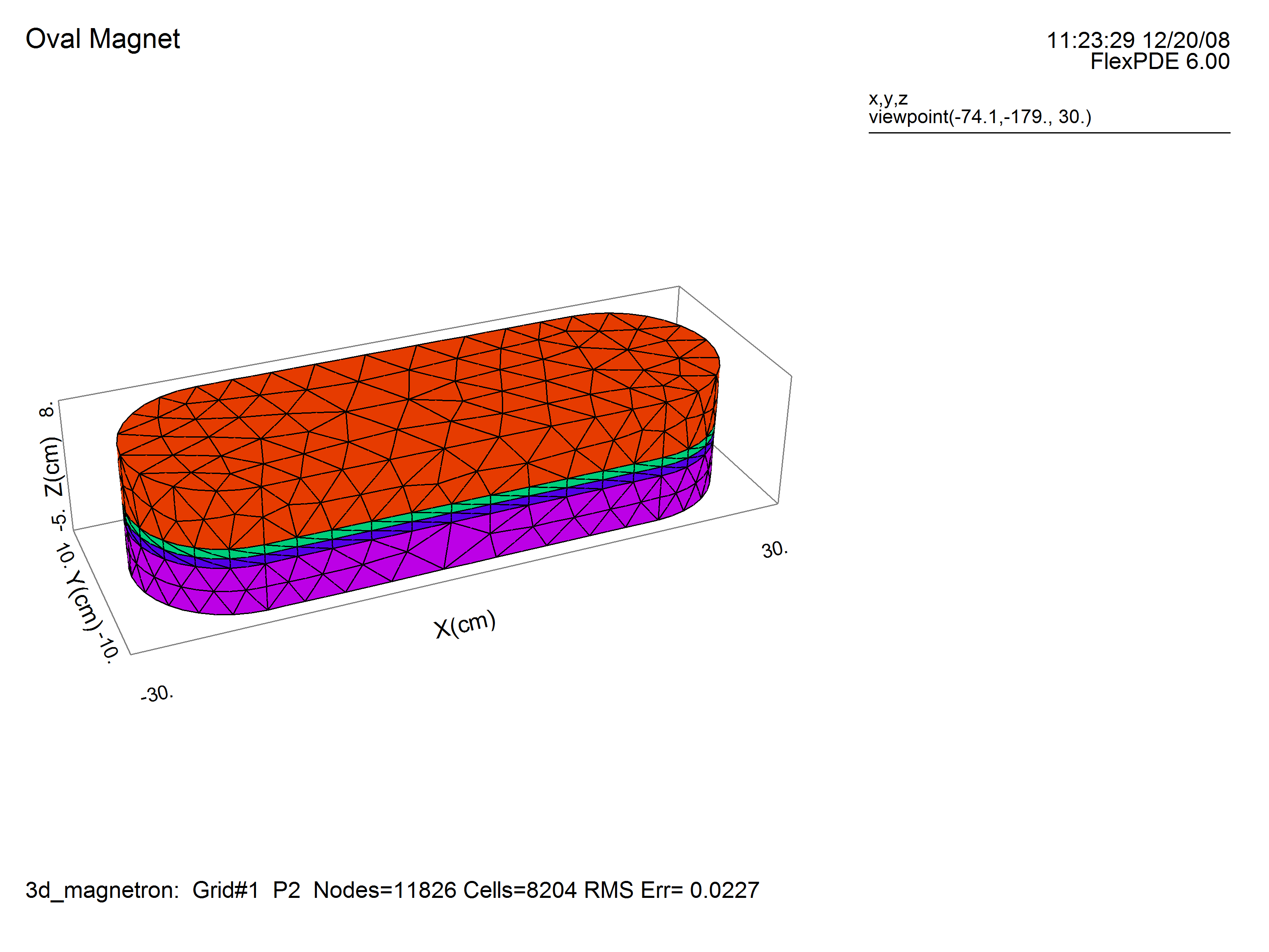
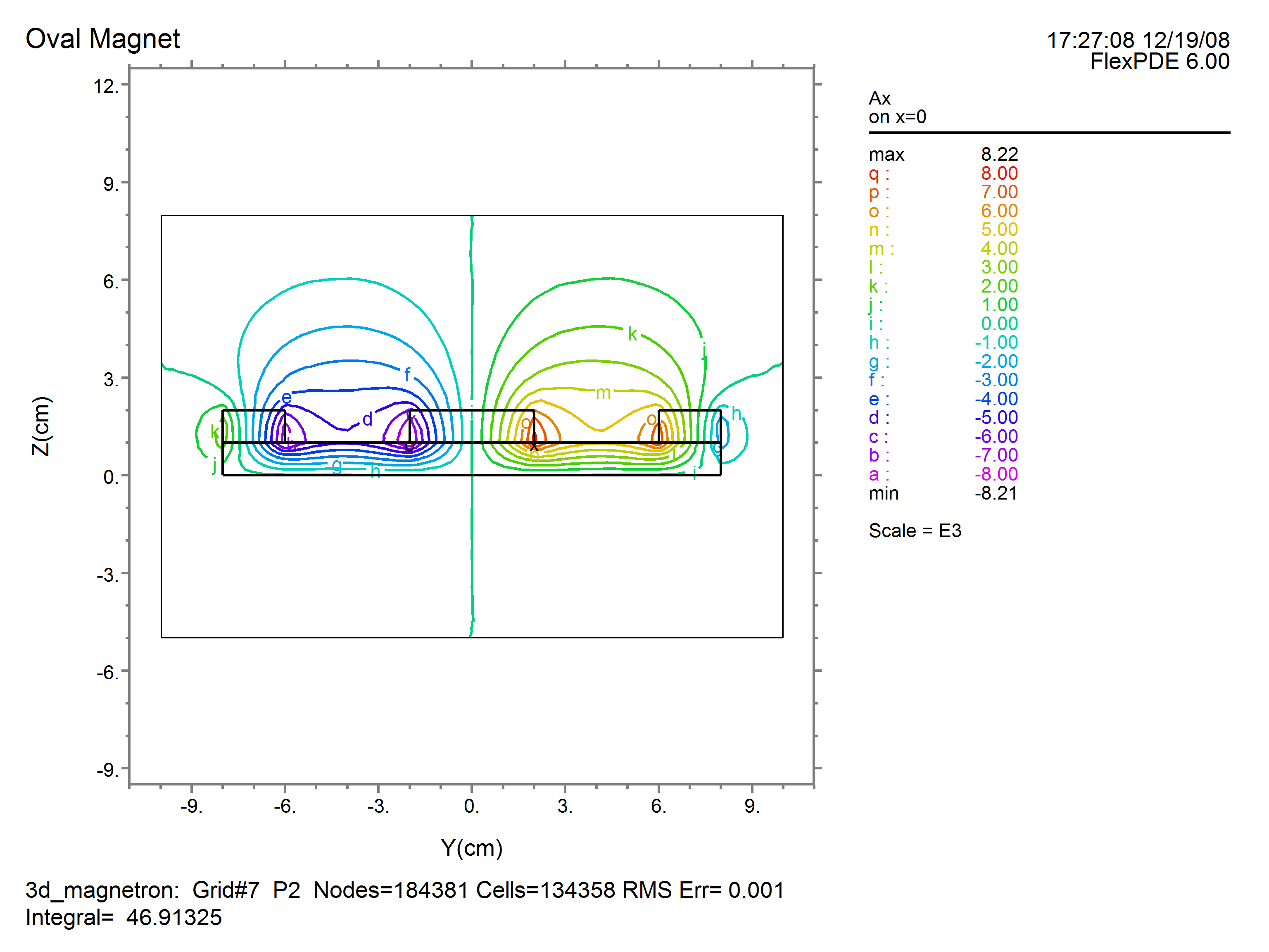
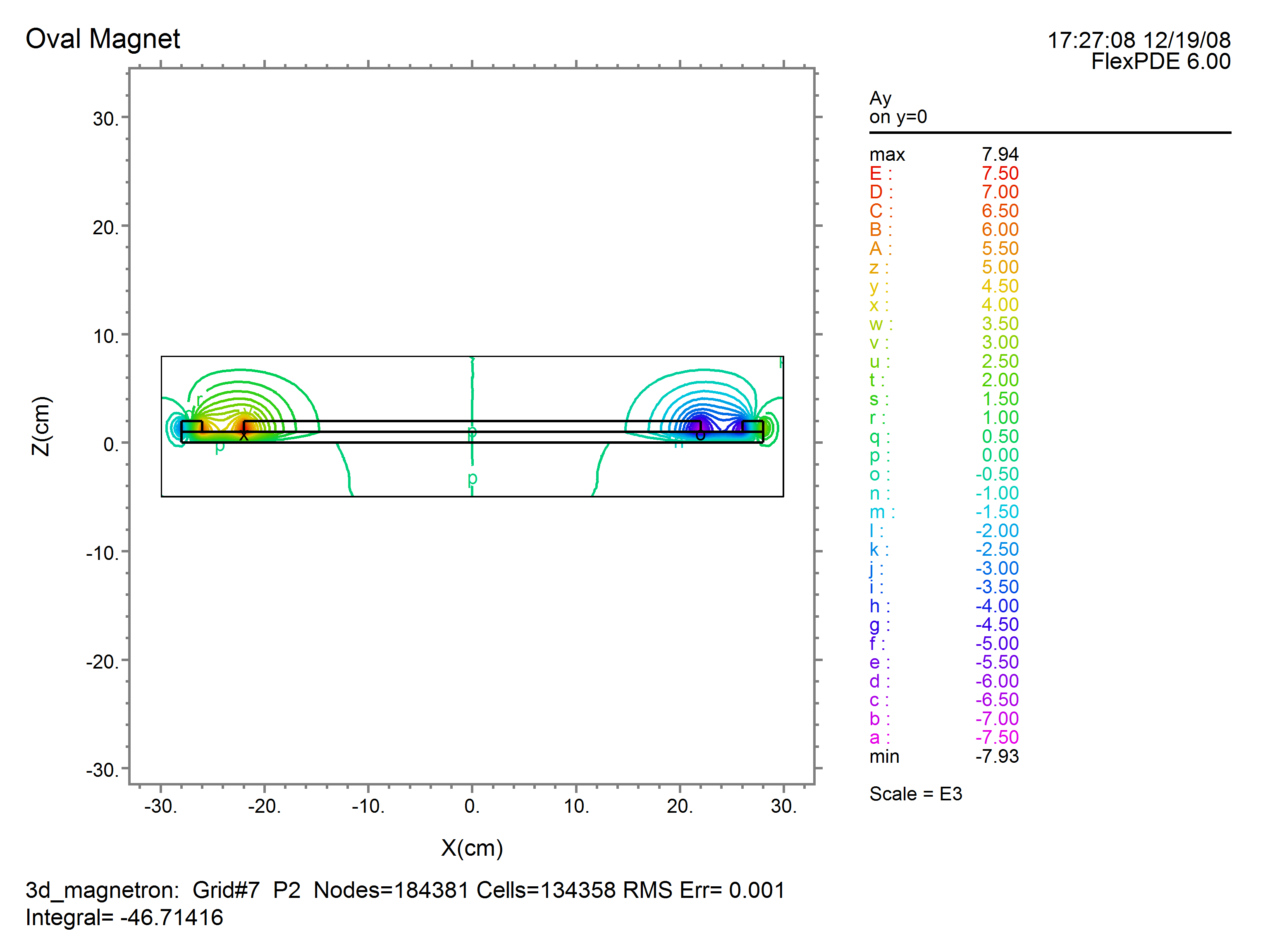
As an example, we will compute the magnetic field in a generic magnetron. In this case, only is applied by the magnets, and as a result will be zero. We will therefore delete from the analysis. The outer and inner magnets are in reversed orientation, so the applied is reversed in sign.

Descriptor 2.3: 3D_Magnetron.pde

TITLE 'Oval Magnet'

COORDINATES

CARTESIAN3

SELECT

alias(x) = "X(cm)"

alias(y) = "Y(cm)"

alias(z) = "Z(cm)"

nodelimit = 40000

errlim=1e-4

VARIABLES

Ax,Ay { assume Az is zero! }

DEFINITIONS

MuMag=1.0 { Permeabilities: }

MuAir=1.0

MuSST=1000

MuTarget=1.0

Mu=MuAir { default to Air }

MzMag = 10000 { permanent magnet strength }

Mz = 0

Nx = vector(0,Mz,0)

Ny = vector(-Mz,0,0)

B = curl(Ax,Ay,0) { magnetic flux density }

Bxx= -dz(Ay)

Byy= dz(Ax) { "By" is a reserved word. }

Bzz= dx(Ay)-dy(Ax)

EQUATIONS

Ax: div(grad(Ax)/mu + Nx) = 0

Ay: div(grad(Ay)/mu + Ny) = 0

EXTRUSION

SURFACE "Boundary Bottom" Z=-5

SURFACE "Magnet Plate Bottom" Z=0

LAYER "Magnet Plate"

SURFACE "Magnet Plate Top" Z=1

LAYER "Magnet"

SURFACE "Magnet Top" Z=2

SURFACE "Boundary Top" Z=8

BOUNDARIES

Surface "boundary bottom"

value (Ax)=0 value(Ay)=0

Surface "boundary top"

value (Ax)=0 value(Ay)=0

REGION 1 { Air bounded by conductive box }

START (20,-10)

value(Ax)=0 value(Ay)=0

arc(center=20,0) angle=180

Line TO (-20,10)

arc(center=-20,0) angle=180

LINE TO CLOSE

REGION 2 { Magnet Plate Perimeter and outer magnet }

LAYER "Magnet Plate"

Mu=MuSST

LAYER "Magnet"

Mu=MuMag

Mz=MzMag

START (20,-8)

arc(center=20,0) angle=180

Line TO (-20,8)

arc(center=-20,0) angle=180

LINE TO CLOSE

REGION 3 { Air }

LAYER "Magnet Plate"

Mu=MuSST

START (20,-6)

arc(center=20,0) angle=180

Line TO (-20,6)

arc(center=-20,0) angle=180

LINE TO CLOSE

REGION 4 { Inner Magnet }

LAYER "Magnet Plate"

Mu=MuSST

LAYER "Magnet"

Mu=MuMag

Mz=-MzMag

START (20,-2)

arc(center=20,0) angle=180

Line TO (-20,2)

arc(center=-20,0) angle=180

LINE TO CLOSE

MONITORS

grid(x,z) on y=0

grid(x,y) on z=1.01

grid(x,z) on y=1

PLOTS

grid(x,y) on z=1.01

grid(y,z) on x=0

grid(x,z) on y=0

contour(Ax) on x=0

contour(Ay) on y=0

vector(Bxx,Byy) on z=2.01 norm

vector(Byy,Bzz) on x=0 norm

vector(Bxx,Bzz) on y=4 norm

contour(magnitude(Bxx,Byy,Bzz)) on z=2.01 LOG

END

Magnetic Materials in 3D

Magnetic Materials in 3D

Descriptor 2.3: 3D_Magnetron.pde