Technical Notes > Applications in Electromagnetics > Electrostatics > Capacitance per Unit Length in 2D Geometry

- Submitted by J.B. Trenholme

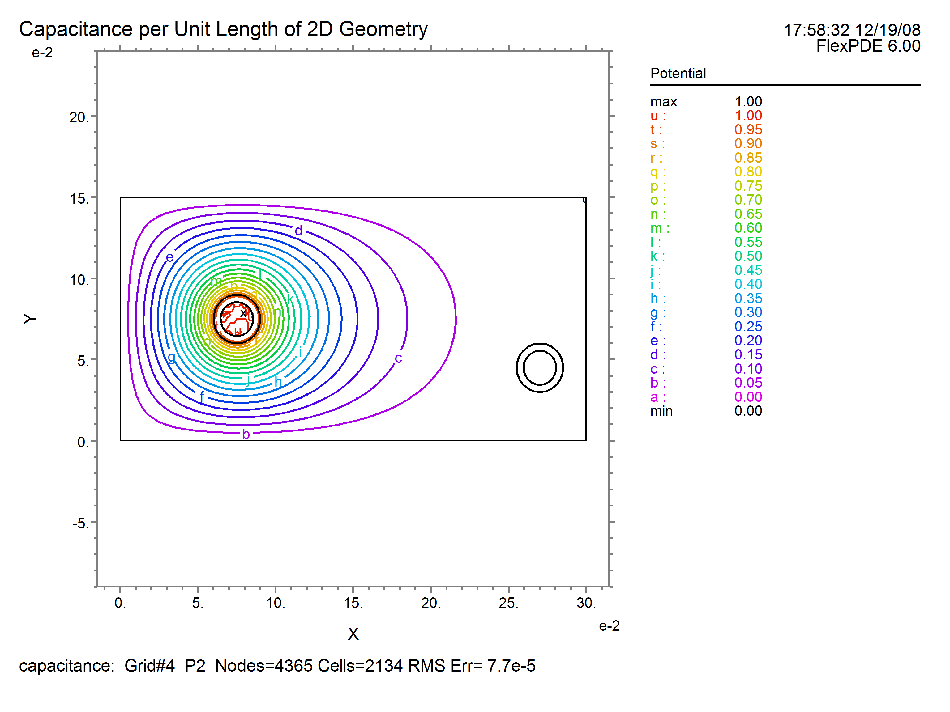
This problem illustrates the calculation of capacitance per unit length in a 2D X-Y geometry extended indefinitely in the Z direction. The capacitance is that between a conductor enclosed in a dielectric sheath and a surrounding conductive enclosure. In addition to these elements, there is also another conductor (also with a dielectric sheath) that is "free floating" so that it maintains zero net charge and assumes a potential that is consistent with that uncharged state.

We use the potential as the system variable, from which we can calculate the electric fieldand displacement , where is the local permittivity and may vary with position.

In steady state, in charge-free regions, Maxwell’s equation then becomes

We impose value boundary conditions on at the surfaces of the two conductors, so that we do not have to deal with regions that contain charge.

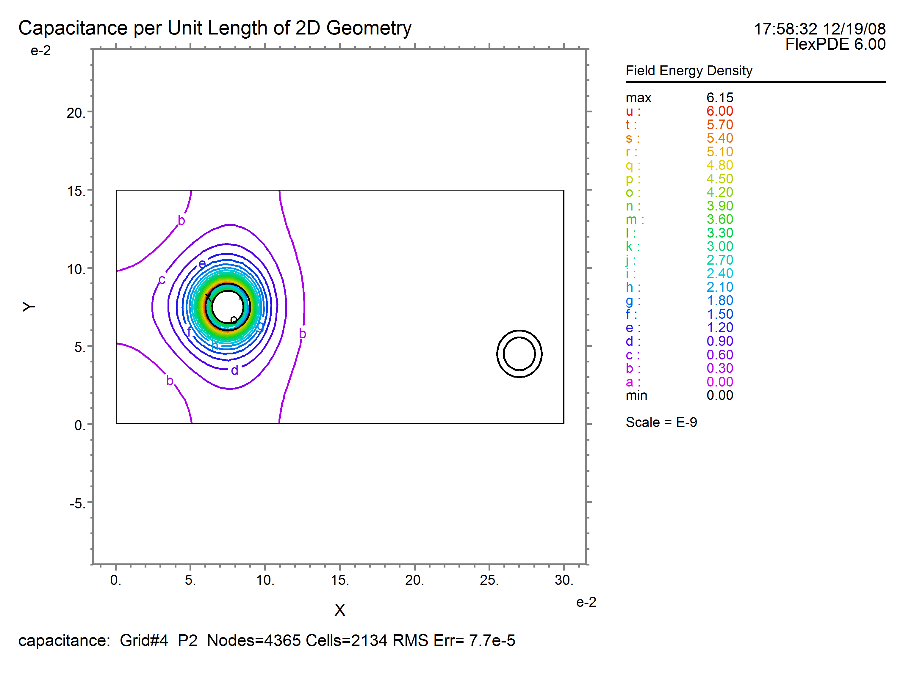
The metal in the floating conductor is "faked" with a fairly high permittivity, which has the effect of driving the interior field and field energy to near zero. The imposition of (default) natural boundary conditions then keeps the field normal to the surface of the conductor, as Maxwell requires. Thus we get a good answer without having to solve for the charge on the floating conductor, which would be a real pain due to its localization on the surface of the conductor.

The capacitance can be found in two ways. If we know the charge on the conductor at fixed potential , we solve

to get. We know because it is imposed as a boundary condition, and we can find from the fact that , where the integral is taken over a surface enclosing a volume and is the total charge in the volume.

Alternatively, we can use the energy relation to get . We find the energy by integrating the energy density over the area of the problem.

Descriptor 1.3: Capacitance.pde

TITLE 'Capacitance per Unit Length of 2D Geometry'

{ 17 Nov 2000 by John Trenholme }

SELECT

errlim 1e-4

thermal_colors on

plotintegrate off

VARIABLES

DEFINITIONS

mm = 0.001 ! meters per millimeter

Lx = 300 * mm ! enclosing box dimensions

Ly = 150 * mm

b = 0.7 ! fractional radius of conductor

! position and size of cable at fixed potential:

x0 = 0.25 * Lx

y0 = 0.5 * Ly

r0 = 15 * mm

x1 = 0.9 * Lx

y1 = 0.3 * Ly

r1 = r0

epsr ! relative permittivity

epsd = 3 ! epsr of cable dielectric

epsmetal = 1000 ! fake metallic conductor

eps0 = 8.854e-12 ! permittivity of free space

eps = epsr * eps0

v0 = 1 ! fixed potential of the cable

! field energy density:

energyDensity = dot( eps * grad( v), grad( v) )/2

EQUATIONS

div( eps * grad( v) ) = 0

BOUNDARIES

region 1 'inside' epsr = 1

start 'outer' ( 0, 0) value( v) = 0

line to (Lx,0) to (Lx,Ly) to (0,Ly) to close

region 2 'diel0' epsr = epsd

start 'dieb0' (x0+r0, y0)

arc ( center = x0, y0) angle = 360

region 3 'cond0' epsr = 1

start 'conb0' (x0+b*r0, y0) value(v) = v0

arc ( center = x0, y0) angle = 360

region 4 'diel1' epsr = epsd

start 'dieb1' ( x1+r1, y1)

arc ( center = x1, y1) angle = 360

region 5 'cond1' epsr = epsmetal

start 'conb1' ( x1+b*r1, y1)

arc ( center = x1, y1) angle = 360

PLOTS

contour( v) as 'Potential'

contour( v) as 'Potential Near Driven Conductor'

zoom(x0-1.1*r0, y0-1.1*r0, 2.2*r0, 2.2*r0)

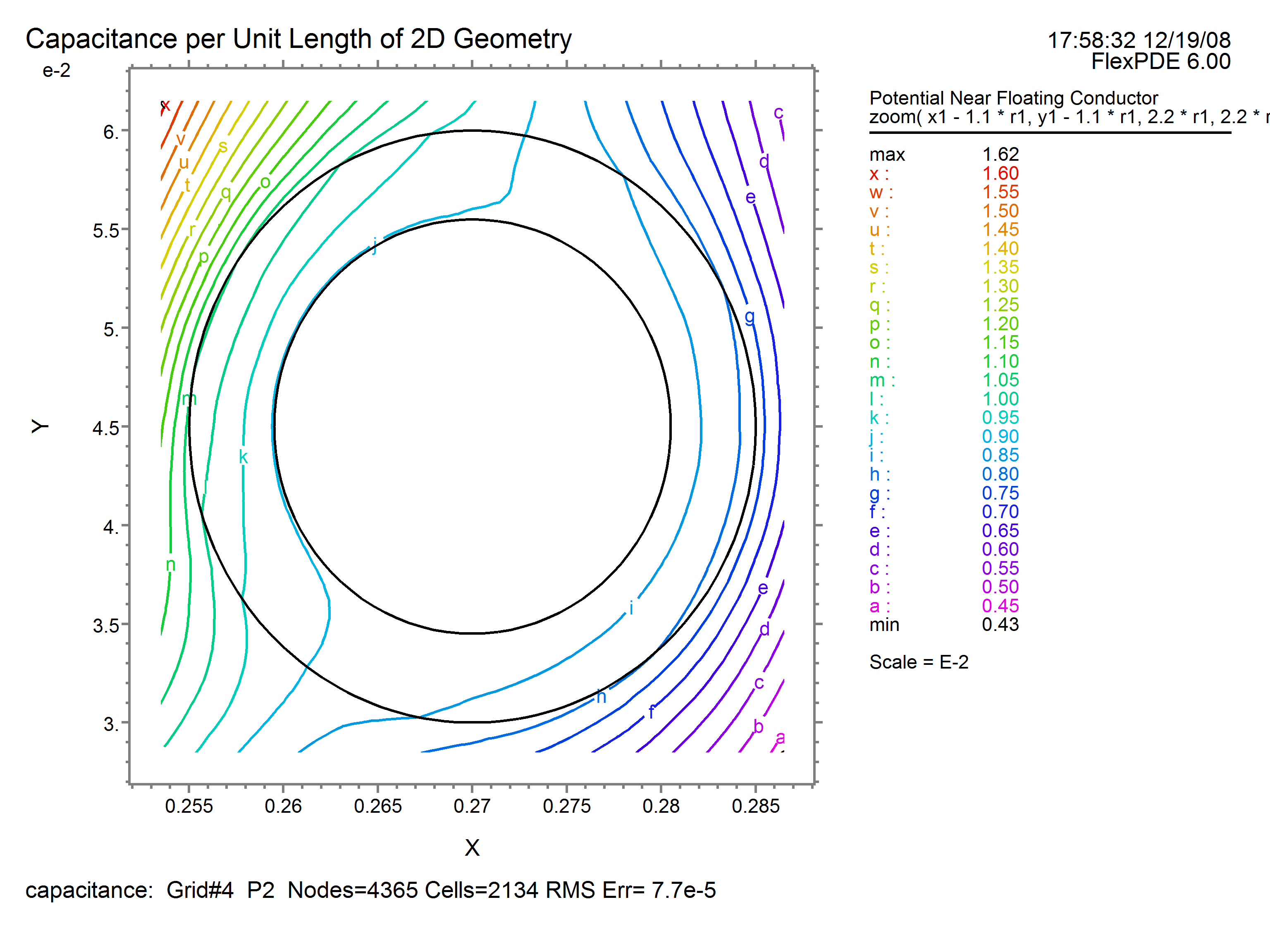
contour( v) as 'Potential Near Floating Conductor'

zoom(x1-1.1*r1, y1-1.1*r1, 2.2*r1, 2.2*r1)

elevation( v) from ( 0,y0) to ( x0, y0)

as 'Potential from Wall to Driven Conductor'

elevation( v) from ( x0, y0) to ( x1, y1)

as 'Potential from Driven to Floating Conductor'

vector( grad( v)) as 'Field'

contour( energyDensity) as 'Field Energy Density'

contour( energyDensity)

zoom( x1-1.2*r1, y1-1.2*r1, 2.4*r1, 2.4*r1)

as 'Field Energy Density Near Floating Conductor'

elevation( energyDensity)

from (x1-2*r1, y1) to ( x1+2*r1, y1)

as 'Field Energy Density Near Floating Conductor'

contour( epsr) paint on "inside"

as 'Definition of Inside'

SUMMARY

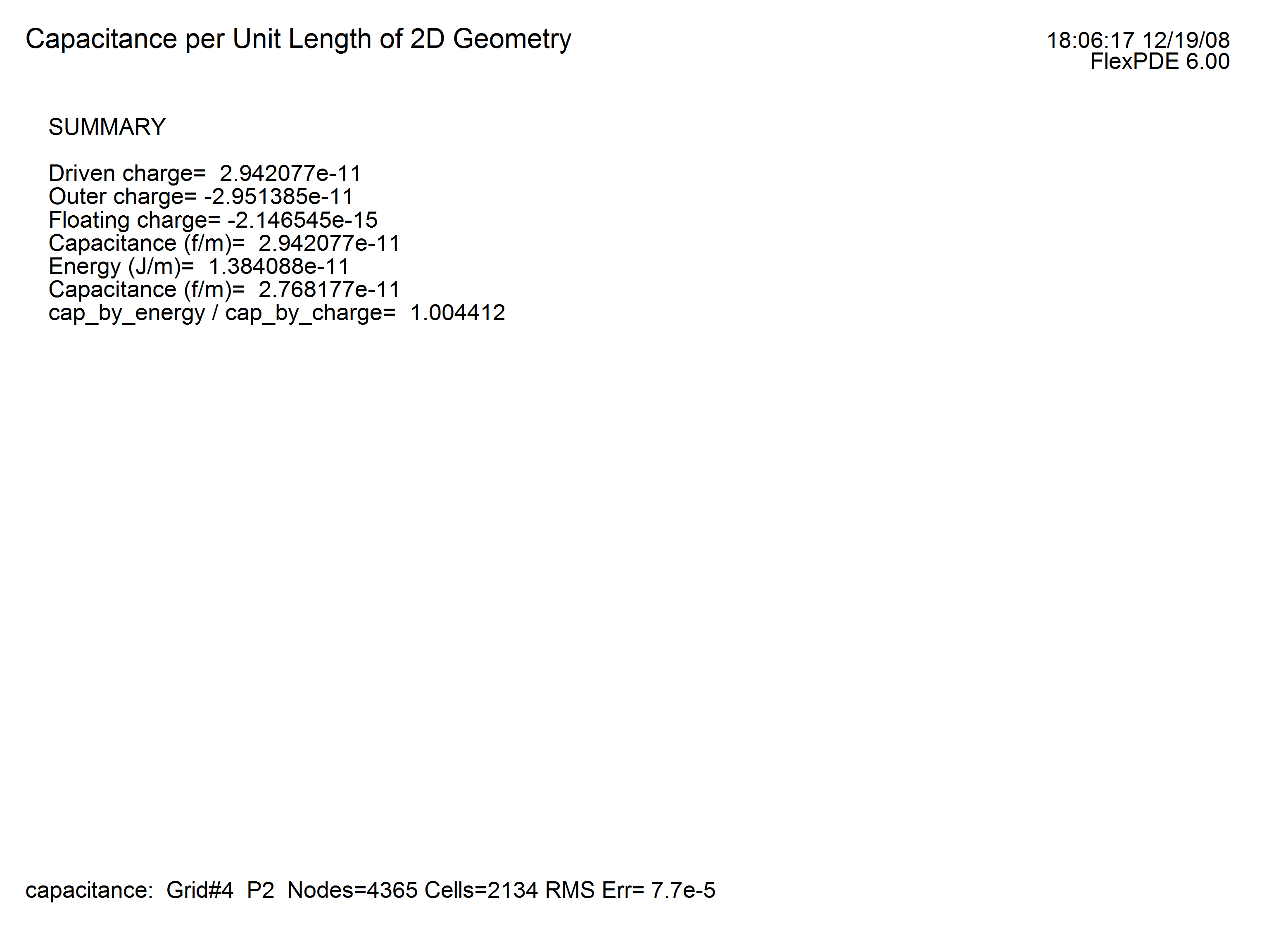
report sintegral(normal(eps*grad(v)),'conb0', 'diel0')

as 'Driven charge'

report sintegral(normal(eps*grad(v)),'outer','inside')

as 'Outer charge'

report sintegral(normal(eps*grad(v)),'conb1','diel1')

as 'Floating charge'

report sintegral(normal(eps*grad(v)),'conb0','diel0')/v0

as 'Capacitance (f/m)'

report integral( energyDensity, 'inside')

as 'Energy (J/m)'

report 2 * integral( energyDensity, 'inside') / v0^2

as 'Capacitance (f/m)'

report 2 * integral(energyDensity)/(v0*

sintegral( normal(eps*grad(v)), 'conb0', 'diel0'))

as 'cap_by_energy / cap_by_charge'

END