Sample Problems > Applications > Chemistry

{ MELTING.PDE

This problem shows the application of FlexPDE to the melting of metal.

We choose as our system variables the temperature, "temp", and the

fraction of material which is solid at any point, "solid".

The temperature is given by the heat equation,

rho*cp*dt(temp) - div(lambda*grad(temp)) = Source

where cp is the heat capacity, rho the density and lambda the conductivity.

The latent heat, Qm, is an amount of heat released as "Solid" changes from

zero to one. We have Qm = integral[0,1]((dH/dSolid)*dSolid), or assuming

dH/dSolid is constant, dH/dSolid = Qm.

Then heat source from freezing is

dH/dt = (dH/dSolid)*(dSolid/dt) = Qm*dt(Solid).

We assume that the solid fraction can be represented by a linear ramp from

one down to zero as the temperature passes from (Tm-T0/2) to (Tm+T0/2).

solid = 1 when temp < Tm-T0

(Tm+T0/2-temp)/T0 when Tm-T0 <= temp <= Tm+T0

0 when temp > Tm+T0

where Tm is the melting temperature, and T0 is a temperature range over

which the melting transition occurs. Since there are no spatial derivatives

in this equation, we introduce a diffusion term with small coefficient to act

as a noise filter.

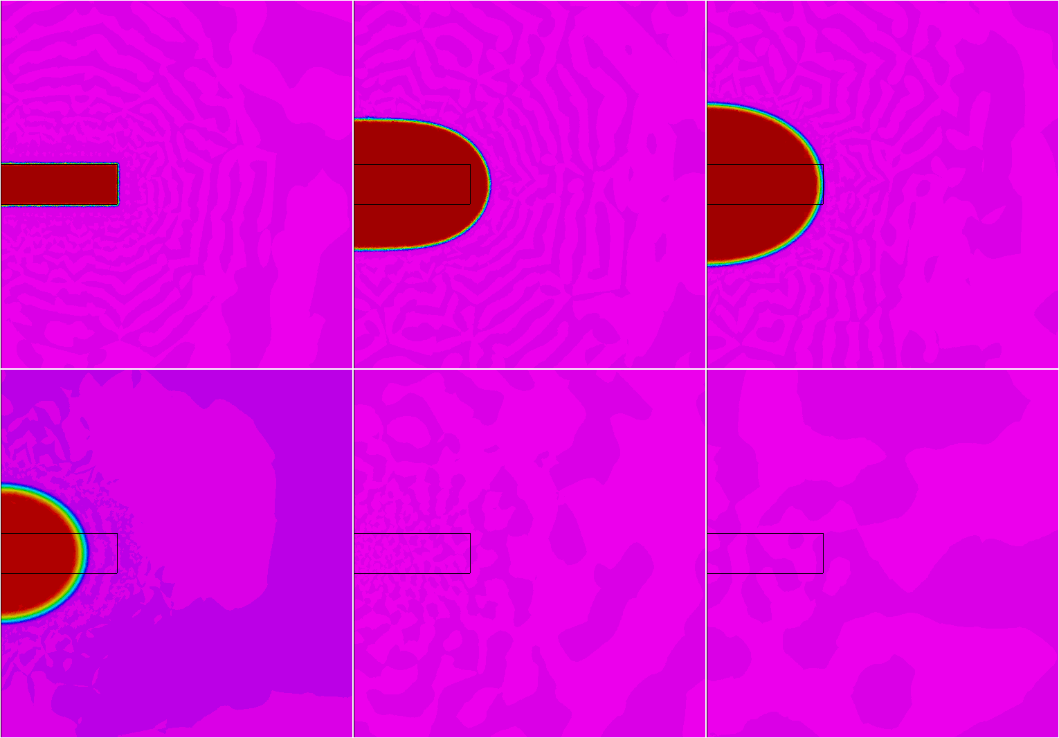
The particular problem addressed here is a disk of cold solid material

immersed in a bath of liquid. The initial temperatures are such that material

first freezes onto the disk, but after equilibrium is reached all the material

is liquid. The outer boundary is insulated.

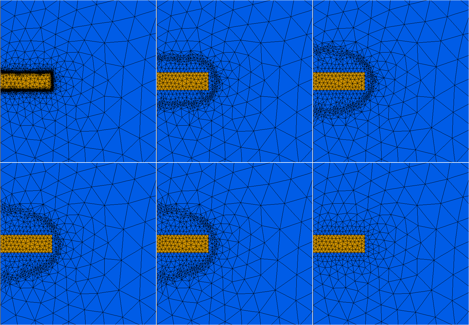
Since the initial condition is a discontinuous distribution, we use a separate

REGION to define the cold initial disk, so that the grid lines will follow the

shape. We also add a FEATURE bounding the disk to help the gridder

define the abrupt transition. SELECT SMOOTHINIT helps minimize

interpolator overshoots.

}

TITLE

'Melting Metal'

COORDINATES

ycylinder('r','z')

SELECT

smoothinit

threads=2

VARIABLES

temp(threshold=1)

solid(threshold=0.01)

DEFINITIONS

Qm= 225000 { latent heat }

Tm=1850 { Melting temperature }

T0= 20 { Melting interval +- T0 }

temp_liq=2000 { initial liquid temperature }

temp_sol=400 { initial solid temperature }

Tinit

R_inf = 0.7 { Domain Radius m}

{ plate }

d=0.05

dd = d/5 { a defining layer around discontinuity }

R_Plate=0.15

K = 30+4.5e-5*(temp-1350)^2 { Conductivity }

rho=2500 { Density kg/m3 }

cp = 700 { heat capacity }

INITIAL VALUES

temp=Tinit

solid = 0.5*erfc((tinit-Tm)/T0)

EQUATIONS

temp: rho*cp*dt(temp) - div(K*grad(temp)) = Qm*dt(solid)

solid: solid - 1e-6*div(grad(solid)) = RAMP((temp-Tm), 1, 0, T0)

BOUNDARIES

region 'Outer'

Tinit = temp_liq

start 'outer' (0,-R_inf)

value(temp)= temp_liq arc(center=0,0) angle 180

natural(temp)=0 line to close

region 'Plate'

Tinit = temp_sol

start(0,0)

mesh_spacing=dd

line to (R_Plate,0) to (R_Plate,d) to (0,d) to close

TIME 0 by 1e-5 to 600

MONITORS

for cycle=10

grid(r,z) zoom (0,-0.1,0.25,0.25)

elevation(temp) from(0.1,-0.1) to (0.1,0.15) range=(0,2000)

elevation(solid) from(0.1,-0.1) to (0.1,0.15) range=(0,1)

PLOTS

for t= 0 1e-4 1e-3 1e-2 0.1 1 10 by 10 to 100 by 100 to 300 by 300 to endtime

contour(temp) range=(0,2000)

contour(temp) zoom (0,-0.2,0.45,0.45) range=(0,2000)

elevation(temp) from(0.1,-0.1) to (0.1,0.15) range=(0,2000)

contour(solid) range=(0,1)

contour(solid) zoom (0,-0.2,0.45,0.45) range=(0,1)

surface(solid) zoom (0,-0.2,0.45,0.45) range=(0,1) viewpoint(1,-1,30)

elevation(solid) from(0.1,-0.1) to (0.1,0.15) range=(0,1)

HISTORIES

history(temp) at (0.051,d/2) (0.075,d/2) (R_plate,d/2)

history(temp) at (0.051,d) (0.075,d) (R_plate,d)

history(solid) at (0.051,d/2) (0.075,d/2) (R_plate,d/2)

history(solid) at (0.051,d) (0.075,d) (R_plate,d)

history(integral(cp*temp+Qm*(1-solid))) as "Total Energy"

END