<< Click to Display Table of Contents >> Navigation:  Sample Problems > Usage > Eigenvalues > vibar

{ VIBAR.PDE

 

 This problem analyzes the standing-wave vibrational modes of an elastic bar.

 

 The equations of Stress/Strain in a material medium can be given as

       dx(Sx) + dy(Txy) + Fx = 0

       dx(Txy) + dy(Sy) + Fy = 0

 

 where Sx and Sy are the stresses in the x- and y- directions,

 Txy is the shear stress, and Fx and Fy are the body forces in the

 x- and y- directions.

 

 In a time-dependent problem, the material acceleration and viscous force

 act as body forces, and are included in a new body force term

       Fx1 = Fx0 - rho*dtt(U) + mu*del2(dt(U))

       Fy1 = Fy0 - rho*dtt(V) + mu*del2(dt(V))

 

 where rho is the material mass density, mu is the viscosity, and U and V

 are the material displacements in the x and y directions.

 

 If we assume that the displacement is harmonic in time (all transients

 have died out), then we can assert

       U(t) = U0*exp(-i*omega*t)

       V(t) = V0*exp(-i*omega*t)

 

 Here U0(x,y) and V0(x,y) are the complex amplitude distributions, and

 omega is the angular velocity of the oscillation.

 

 Substituting this assumption into the stress equations and dividing out

 the common exponential factors, we get (implying U0 by U and V0 by V)

       dx(Sx) + dy(Txy) + Fx0 + rho*omega^2*U - i*omega*mu*del2(U) = 0

       dx(Txy) + dy(Sy) + Fy0 + rho*omega^2*V - i*omega*mu*del2(V) = 0

 

 All the terms in this equation are now complex.  Separating into real

 and imaginary parts gives

       U = Ur + i*Ui

       Sx = Srx + i*Six

       Sy = Sry + i*Siy

       etc...

 

 Expressed in terms of the (assumed real) constitutive relations of the material,

       Srx = [C11*dx(Ur) + C12*dy(Vr)]

       Sry = [C12*dx(Ur) + C22*dy(Vr)]

       Trxy = C33*[dy(Ur) + dx(Vr)]

       etc...

 

 The final result is a set of four equations in Ur,Vr,Ui and Vi.

   Ur: dx(Srx) + dy(Trxy) + rho*omega^2*Ur + omega*mu*del2(Ui) = 0

   Ui: dx(Six) + dy(Tixy) + rho*omega^2*Ui - omega*mu*del2(Ur) = 0

   Vr: dx(Trxy) + dy(Sry) + rho*omega^2*Vr + omega*mu*del2(Vi) = 0

   Vi: dx(Tixy) + dy(Siy) + rho*omega^2*Vi - omega*mu*del2(Vr) = 0

 

 In the absence of viscous effects, these equations separate, with no imaginary

 terms appearing in the real equations, and vice versa.

 

 We can therefore solve only for the real components Ur and Vr, which we

 will continue to refer to as U and V.

 

 Solving the eigenvalue system  

   U:        dx(Sx)  + dy(Txy) + lambda*rho*U = 0

   V:        dx(Txy)   + dy(Sy) + lambda*rho*V = 0

 we find the resonant frequencies lambda = omega^2 together with the  

 corresponding spatial amplitude distributions Uand V.

 

 In order to quantify the "natural" (or "load") boundary condition mechanism,

 we can write the equations as

   U:     div(P) + lambda*rho*U = 0

   V:     div(Q) + lambda*rho*V = 0

 where P = [Sx,Txy]

 and   Q = [Txy,Sy]

 

 The natural (or "load") boundary condition for the U-equation defines the

 outward surface-normal component of P, while the natural boundary condition

 for the V-equation defines the surface-normal component of Q. Thus, the

 natural boundary conditions for the U- and V- equations together define

 the surface load vector.

 

 On a free boundary, both of these vectors are zero, so a free boundary

   nu = 0.3           { Poisson's Ratio }  

   E  = 20             { Young's Modulus for Steel x10^11(dynes/cm^2) }  

   G  = 0.5*E/(1+nu)  

   rho = 7.8           { Density (g/cm^3) }  

 

  { plane strain coefficients }  

   E1 = E/((1+nu)*(1-2*nu))  

   C11 = E1*(1-nu)  

   C12 = E1*nu  

   C22 = E1*(1-nu)  

   C33 = E1*(1-2*nu)/2  

 

  { Stresses }  

   Sx = (C11*dx(U) + C12*dy(V))      

   Sy = (C12*dx(U) + C22*dy(V))  

   Txy = C33*(dy(U) + dx(V))  

 

   mag=0.05  

 

initial values  

   U = 0  

   V = 0  

 

equations               { define the displacement equations }  

   U:  dx(Sx)  + dy(Txy) + lambda*rho*U = 0  

   V:  dx(Txy)  + dy(Sy) + lambda*rho*V = 0  

 

constraints

 line_integral(V,"mount")=0   { constrain the net right end y-motion to be zero }

 

boundaries

  region 1

    start (0,-hW)

 

    { free boundary on bottom, no normal stress }

    load(U)=0     load(V)=0       line to (L,-hW)

 

 

    { clamp the right end x-motion }

     label 'mount'

    value(U) = 0     line to (L,hW)

     endlabel 'mount'

 

    { free boundary on top, no normal stress }

    load(U)=0     load(V)=0       line to (0,hW)

 

    load(U) = 0   load(V) = 0     line to close

 

monitors  

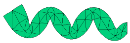
  grid(x+mag*U,y+mag*V)   as "deformation"   { show final deformed grid }  

plots  

  grid(x+mag*U,y+mag*V)   as "deformation"   { show final deformed grid }  

  contour(U) as "X-Displacement(M)"  

  contour(V) as "Y-Displacement(M)"  

 

end