Sample Problems > Applications > Fluids

{ FLOWSLAB.PDE

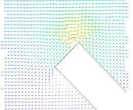
This problem considers the laminar

flow of an incompressible, inviscid

fluid past an obstruction.

We assume that the flow can be

represented by a stream function, PSI,

such that the velocities, U in the

x-direction and V in the y-direction,

are given by:

U = -dy(PSI)

V = dx(PSI)

The flow can then be described by the

equation

div(grad(PSI)) = 0.

The contours of PSI describe the flow

trajectories of the fluid.

The problem presented here describes

the flow past a slab tilted at

45 degrees to the flow direction. The

left and right boundaries are held

at PSI=y, so that U=-1, and V=0.

}

title "Stream Function Flow past 45-degree slab"

variables

psi { define PSI as the system variable }

definitions

a = 3; b = 3 { size of solution domain }

len = 0.5 { projection of length/2 }

wid = 0.1 { projection of width/2 }

psi_far = y { solution at large x,y }

equations { the equation of continuity: }

psi : div(grad(psi)) = 0

boundaries

region 1 { define the domain boundary }

start(-a,-b) { start at the lower left }

value(psi)= psi_far { impose U=-1 on the outer boundary }

line to (a,-b) { walk the boundary Counter-Clockwise }

to (a,b)

to (-a,b)

to close { return to close }

start(-len-wid,len-wid) { start at upper left corner of slab }

value(psi)=0 { specify no flow on the slab surface }

line to (-len+wid,len+wid){ walk around the slab CLOCKWISE for exclusion }

to (len+wid,-len+wid)

to (len-wid,-len-wid)

to close { return to close }

monitors

contour(psi) { show the potential during solution }

plots { write hardcopy files at termination }

grid(x,y) { show the final grid }

grid(x,y) zoom(-1,0,1,1) { magnify gridding at corner }

contour(psi) as "stream lines" { show the stream function }

vector(-dy(psi),dx(psi)) as "flow" { show the flow vectors }

vector(-dy(psi),dx(psi)) as "flow" zoom(-1,0,1,1)

end

flowslab

flowslab