<< Click to Display Table of Contents >> Navigation:  Sample Problems > Applications > Fluids > viscous

{  VISCOUS.PDE

 

 This example shows the application of FlexPDE to problems in

 viscous flow.

 

 The Navier-Stokes equation for steady incompressible flow in two

 cartesian dimensions is  

       dens*(dt(U) + U*dx(U) + V*dy(U)) = visc*del2(U) - dx(P) + dens*Fx

       dens*(dt(V) + U*dx(V) + V*dy(V)) = visc*del2(V) - dy(P) + dens*Fy  

 together with the continuity equation  

       div[U,V] = 0  

 where

       U and V are the X- and Y- components of the flow velocity

       P is the fluid pressure

       dens is the fluid density

       visc is the fluid viscosity

       Fx and Fy are the X- and Y- components of the body force.

 

 In principle, the third equation enforces incompressible mass conservation,

 but the equation contains no reference to the pressure, which is nominally

 the remaining variable to be determined.

 

 In practice, we choose to solve a "slightly compressible" system by defining a

 hypothetical equation of state  

   p(dens) = p0 + L*(dens-dens0)  

 where p0 and dens0 represent a reference density and pressure, and L is a large

 number representing a strong response of pressure to changes of density.  L is

 chosen large enough to enforce the near-incompressibility of the fluid, yet not

 so large as to erase the other terms of the equation in the finite precision

 of the computer arithmetic.

 

 The compressible form of the continuity equation is  

   dt(dens) + div(dens*U) = 0  

 which, together with the equation of state yields  

   dt(p) = -L*dens0*div(U)

 

 In steady state, we can replace the dt(p) by -div(grad(p))

    [see Help | Tech Notes | Smoothing Operators in PDEs"],

 resulting in the final pressure equation:  

   div(grad(p)) = M*div(U)  

 Here M has the dimensions of density/time or viscosity/distance^2.

 

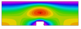
 The problem posed here shows flow in a 2D channel blocked by a bar of square

 cross-section.  The channel is mirrored on the bottom face, and only the upper

 half is computed.

 

 We have chosen a "convenient" value of M, one that gives good

 accuracy in reasonable time.  The user can alter this value to find one

 which is satisfactory for his application.

 

 We have included three elevation plots of X-velocity, at the inlet, center

 and outlet of the channel.  The integrals presented on these plots show the

 consistency of mass transport across the channel.

 

}  

 

title 'Viscous flow in 2D channel, Re < 0.1'  

 

 

  vxx = (p0/(2*visc*Lx))*(Ly-y)^2 { open-channel x-velocity }  

 

  rball=0.25  

  cut = 0.05   { value for bevel at the corners of the obstruction }  

 

  pfactor = staged(1,10,100,1000)

  penalty = pfactor*visc/rball^2   { "equation of state" }  

  Re = globalmax(speed)*(Ly/2)/(visc/dens)  

 

initial values  

  u = 0.5*vxx  v = 0  p = p0*x/Lx  

 

equations  

  u:  visc*div(grad(u)) - dx(p) = dens*(u*dx(u) + v*dy(u))  

  v:  visc*div(grad(v)) - dy(p) = dens*(u*dx(v) + v*dy(v))  

  p:  div(grad(p)) = penalty*(dx(u)+dy(v))  

 

boundaries  

  region 1  

    start(0,0)  

      { unspecified boundary conditions default to LOAD=0 }  

      value(v)=0   line to (Lx/2-rball,0)  

      value(u)=0   line to (Lx/2-rball,rball) bevel(cut)  

                  line to (Lx/2+rball,rball) bevel(cut)  

                  line to (Lx/2+rball,0)  

      load(u)=0   line to (Lx,0)  

      value(p)=p0 line to (Lx,Ly)  

      value(u)=0   load(p)=0   line to (0,Ly)  

      load(u)=0   value(p)=0 line to close  

 

monitors  

  contour(speed) report(Re)  

 

plots  

  grid(x,y)  

  contour(u) report(Re)  

  contour(v) report(Re)  

  contour(speed) painted report(Re)  

  vector(u,v) as "flow"   report(Re)  

  contour(p) as "Pressure" painted  

  contour(dx(u)+dy(v)) as "Continuity Error"  

  contour(p) zoom(Lx/2,0,1,1) as "Pressure"  

  elevation(u) from (0,0) to (0,Ly)  

  elevation(u) from (Lx/2,0) to (Lx/2,Ly)  

  elevation(u) from (Lx,0) to (Lx,Ly)  

 

end