<< Click to Display Table of Contents >> Navigation:  Sample Problems > Usage > Eigenvalues > drumhead

{ DRUMHEAD.PDE  

 

   *******************************************************************

   This example illustrates the use of FlexPDE in Eigenvalue problems, or

   Modal Analysis.

   *******************************************************************

 

   The two-dimensional initial-boundary value problem associated with the

   scalar wave equation can be written as  

       c^2*del2(u) - dtt(u) = 0  

   with accompanying initial values and boundary conditions  

       u = f(s,t)              on S1

       dn(u) + a*u = g(s,t)    on S2.

 

   If we assume that solutions have the form  

       u(x,y,t) = exp(i*w*t)*v(x,y)  

   then the equation becomes  

       del2(v) + lambda*v = 0  

   with lambda = (w/c)^2, and with boundary conditions  

       v = 0                   on S1

       dn(v) + a*v = 0         on S2.

 

   The values of lambda for which this system has a non-trivial solution

   are known as the eigenvalues of the system, and the corresponding solutions

   are known as the eigenfunctions or vibration modes of the system.

 

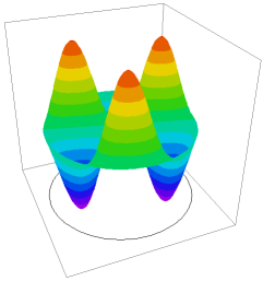
   In this problem, we determine the eight lowest-energy vibrational modes of

   a circular drumhead, clamped on the periphery.

 

   This problem can be solved analytically.  The solutions are of the form  

       v = Jn(r*jnm)*exp(i*n*theta),  

   where Jn is the Bessel function of order n,

         jnm is the m-th root of Jn.

 

   The eigenvalues are then just the sequence of jnm^2. In increasing order :

       5.783186, 14.68197, 14.68197, 26.37459, 26.37459, 30.471262, 40.70644, 40.70644

 

   With default errlim, FlexPDE in the current test gives results within 0.01%.

}  

 

title "Vibrational modes of a drumhead"  

 

select  

    { Define the number of vibrational modes desired.

      The appearance of this selector tells FlexPDE

      to perform an eigenvalue calculation }  

    modes=8    

 

Definitions

    ecorrect = ARRAY(5.783186, 14.68197, 14.68197, 26.37459, 26.37459, 30.471262, 40.70644, 40.70644)