<< Click to Display Table of Contents >> Navigation:  Sample Problems > Usage > Functions > sum

{ SUM.PDE  

 

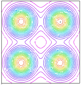
 This example demonstrates the use of the SUM function.

 It poses a heatflow problem with a heat source made up of four

 gaussians.  The source is composed by a SUM over gaussians

 referenced to arrays of center coordinates.

 

}  

title 'Sum test'  

 

Variables  

   u  

 

definitions  

   k = 1  

   u0 = 1-x^2-y^2     { boundary forced to parabolic values }  

   xc = array(-0.5,0.5,0.5,-0.5) { arrays of source spot coordinates }  

   yc = array(-0.5,-0.5,0.5,0.5)  

   s = sum( i, 1, 4, exp(-10*((x-xc[i])^2+(y-yc[i])^2)) )       { summed Gaussian source }