<< Click to Display Table of Contents >> Navigation:  User Guide > Addressing More Difficult Problems > Natural Boundary Conditions > An Example of a Flux Boundary Condition

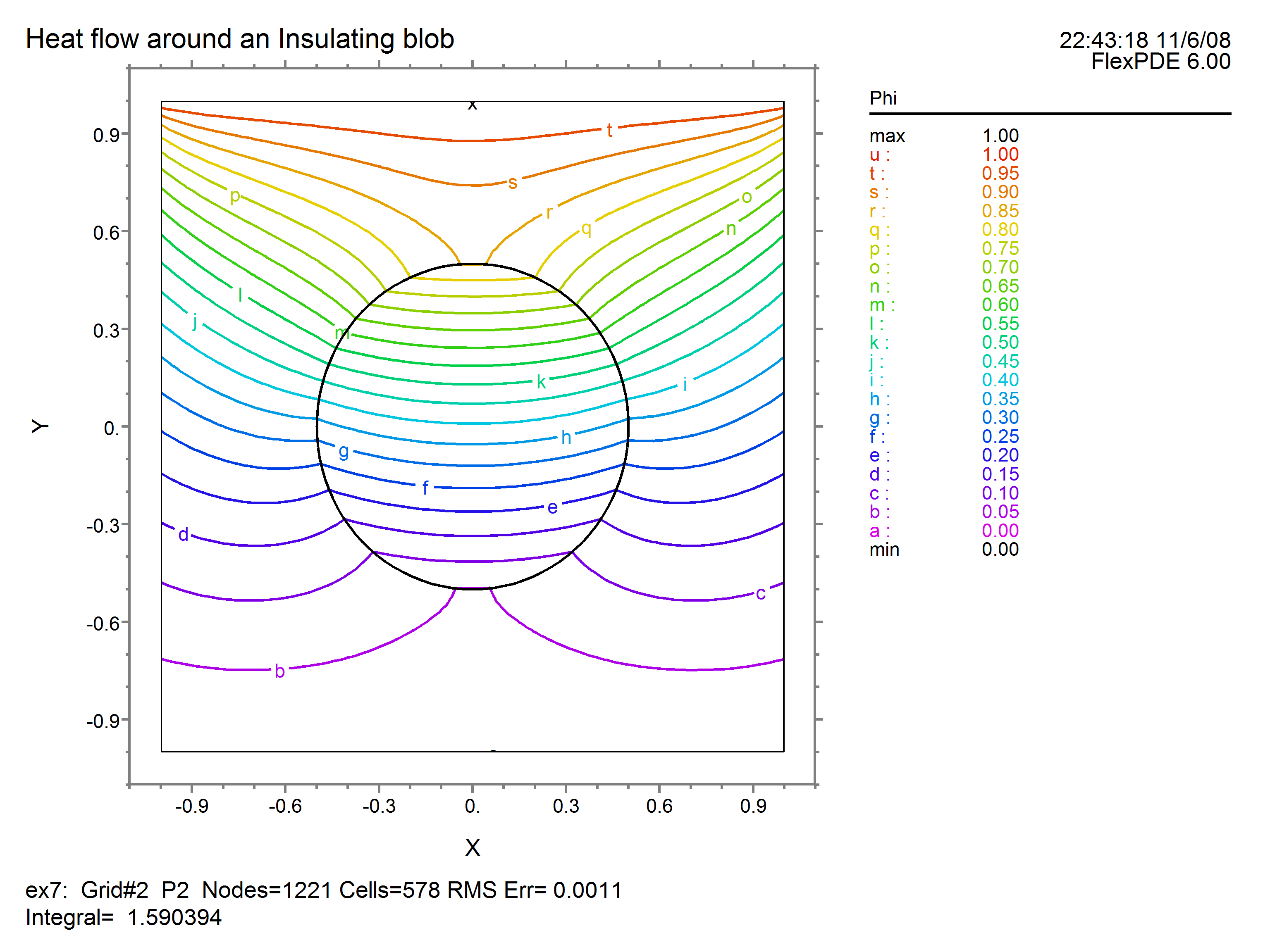
Let us return again to our heat flow test problem and investigate the effect of the Natural boundary condition.   As originally posed, we specified Natural(Phi)=0 on both sidewalls.  This corresponds to zero flux at the boundary.  Alternatively, a convective cooling loss at the boundary would correspond to a flux

Flux = -K*grad(Phi) = Phi – Phi0

 

where Phi0 is a reference cooling temperature.  With convectively cooled sides, our boundary specification looks like this (assuming Phi0=0):

 

REGION 1 'box'

START(-1,-1)

VALUE(Phi)=0                LINE TO (1,-1)

NATURAL(Phi)=Phi        LINE TO (1,1)

VALUE(Phi)=1                LINE TO (-1,1)

NATURAL(Phi)=Phi        LINE TO CLOSE

 

The result of this modification is that the isotherms curve upward: